Coordinate System
· Describe each optical surface location by means of the coordinates (X,Y,Z in the lab frame) of its vertex (pt. at which the surface cuts its own axis)
· Orientation of surface can be changed by
v TILT – pivots a surface around its +x axis
v PITCH – rotates around its +y axis
v ROLL – rotates around the +z axis (see page #32 of manual for visual representation)
Ray Coordinates
Three parameters describe the direction of each ray segment: U, V, and W which are the X, Y, and Z components of the unit-length vector that points in the direction of the ray. In all cases you need to have U2 + V2 + W2 = 1.00. They are referred to as direction cosines due to the fact that each is the cosine of the angle between the ray and its coordinate axis. (U=cos a, V=cos b W=cos g where a, b, g are the angles between the rays and the x, y and z axes respectively)
Example
· A ray headed in the +z direction has U=0, V=0, and W=1.
· A ray headed in the –y direction has U=0, V=-1, and W=0.
· A ray headed 37 degrees away from the +z direction towards the +x direction has U=0.6, V=0 and W=0.8.
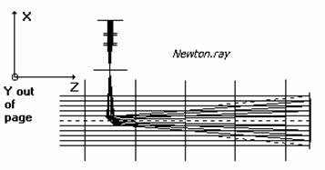
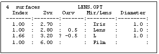 Optics Tables: Example:
Text files organized on a line-by-line basis and can be
edited with some useful functions (see page #77). You need three components to an optics file:
v title line (to include the # of surfaces and an appropriate title and maybe other relevant info.)
v
column
header line (fully programmable with a listing included on page )
v ruler line (set the demarcation of the fields specifying how many digits are allocated to each column.)
Information in the MIRROR/LENS surface identity column tells the program how to calculate ray direction changes at each surface.
Surface TYPES:
|
M, m |
Mirror surface |
G
|
Transmission grating |
|
L, l, blank |
Lens surface (default) |
g |
Reflection grating |
|
I, I |
Iris |
tir |
Total internal reflector |
|
Fresnel |
Fresnel mirror |
retro |
Retroreflector |
|
fresnel |
Fresnel lens |
other |
Phantom: no ray deviation |
The column headers can be customized to fit the specific simulation (detailed description of each is found on page # 38)
Tags – character appearing exactly beneath a field separator. (?,>,<, etc. see page #45 for details) which may be used in flagging critical parameters to be used with AUTOADJUST in making slight changes to these parameters when needed.
Surface
Profiles
 Each spherical surface is described by a
numerical value in the curvature (C) column whose value is the
reciprocal of the radius of curvature
(R), and zero if the surface is flat (i.e. C=1/R). It is positive if
the surface curves towards the +z direction or negative for –z direction.
Each spherical surface is described by a
numerical value in the curvature (C) column whose value is the
reciprocal of the radius of curvature
(R), and zero if the surface is flat (i.e. C=1/R). It is positive if
the surface curves towards the +z direction or negative for –z direction.
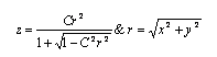
In local coordinates, the equation of a spherical surface with curvature C is:
Here r represents the radial distance from the axis of the
surface.![]()
A SHAPE column can be added to an optics table to specify the conic class of aspheric surfaces.
Surface SHAPES:
shape < 0.0 hyperboloid
shape = 0.0 paraboloid
0 < shape < 1.0 prolate ellipsoid
shape = 1.0 sphere
shape > 1.0 oblate ellipsoid