


Next: About this document ...
PHY294H - Lecture 9
Recommended problems for Lecture 9: 25.7, 25.16, 25.18
Recommended reading for Lecture 10: pp 676-689
A distribution of point charges
Since superposition holds for the electric field, it also holds for
the electric potential. If we have a set of charges  . The
electric field at position
. The
electric field at position  , which is at vector distance
  from charge is given by a vector superposition
of the electric fields due to each of the charges .
In a similar way, the electric potential due to this
distribution of charges is given by,
from charge is given by a vector superposition
of the electric fields due to each of the charges .
In a similar way, the electric potential due to this
distribution of charges is given by,
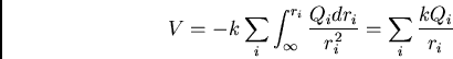 |
(1) |
The nice thing about this superposition is that it is a scalar.
Furthermore, it is possible to find the electric field
from the potential, as we now demonstrate.
Finding the electric field from the potential
It is easier to find the potential due to a set of
point charges than it is to find the electric field
directly. It would therefore be
very nice if we could find the electric field from the
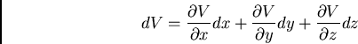
potential. This is actually quite straightforward. The
electric field is given by,
 |
(2) |
However we also know that the  can be written as,
 |
(3) |
So we find,
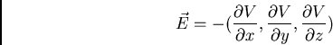 |
(4) |
This is written more succinctly as,
 |
(5) |
where
 is the gradient operator. Its form depends on the
co-ordinate system we choose. For the moment we
only need cartesion co-ordinates, where the gradient
is given by,
is the gradient operator. Its form depends on the
co-ordinate system we choose. For the moment we
only need cartesion co-ordinates, where the gradient
is given by,
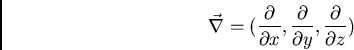 |
(6) |
Another way to visualize the relation between the
electric potential and the electric potential is
to draw equipotential surfaces. On an equipotential
surface, the electric potential is a constant. If
the electric potential is a constant, then
the electric field along the equipotential surface
is zero. This means that the electric field is
perpendicular to the equipotential surface. This
gives us another way of visualizing electric
field lines as well.
A point charge
The electric field is given by,
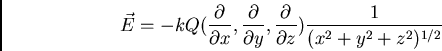 |
(7) |
Thus,
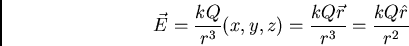 |
(8) |
The electric potential due to a dipole
Consider a dipole lying on the x-axis, with the positive charge
at  and the negative charge at
  . The charges
have magnitude
. The charges
have magnitude  . A point in the x-y plane is defined
by its radial distance to the origin,
. A point in the x-y plane is defined
by its radial distance to the origin,  , and by an angle
 between the direction
  and the x-axis.
We want to find the electric potential due to the dipole
as a function,
and the x-axis.
We want to find the electric potential due to the dipole
as a function,  . The potential is,
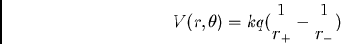 |
(9) |
where,
 |
(10) |
and
 |
(11) |
Using these expressions, we rewrite Eq. (8) as,
![\begin{displaymath}
V(r,\theta) = {kq \over (({d\over 2})^2 + r^2)^{1/2} }
[({1\...
...{1\over 1 +{dr\over ({d\over 2})^2 + r^2} cos{\theta}})^{1/2}]
\end{displaymath}](img24.png) |
(12) |
At long distances where
 , we can use the
expansions,
, we can use the
expansions,
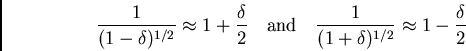 |
(13) |
This yields,
![\begin{displaymath}
V(r>>d,\theta) = { kq \over r}[1 +
{d cos(\theta)\over 2r} - (1- {d cos(\theta)\over 2r})]
\end{displaymath}](img27.png) |
(14) |
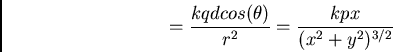 |
(15) |
where  is the magnitude of the dipole moment and we have
used
is the magnitude of the dipole moment and we have
used
 .
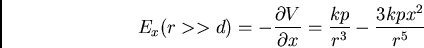
The electric field is given by,
.
The electric field is given by,
|
(16) |
which implies that,
 |
(17) |
 |
(18) |
 |
(19) |
This should be compared with the result we calculated for the
electric field at  ,
,  and
and 
The electric potential energy of a charge distribution
The potential energy of a charge
at position is
 .
A different question is: What is the potential
energy of a distribution of charges, that is, what
is the potential energy stored in a distribution of
charges. The potential energy stored in a distribution
of charges is equal to the work done in setting up the
distribution of charges, provided there is no
dissipation and no kinetic energy is generated. To set up a
distribution of charges at positions ,
we need to bring each of the charges in from infinity
and place it at its allocated position. The work required
to place the first charge is zero (no other charges
are there yet). The work required to place the second
charge is
.
A different question is: What is the potential
energy of a distribution of charges, that is, what
is the potential energy stored in a distribution of
charges. The potential energy stored in a distribution
of charges is equal to the work done in setting up the
distribution of charges, provided there is no
dissipation and no kinetic energy is generated. To set up a
distribution of charges at positions ,
we need to bring each of the charges in from infinity
and place it at its allocated position. The work required
to place the first charge is zero (no other charges
are there yet). The work required to place the second
charge is  , where
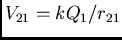 is the
electric potential at position
is the
electric potential at position  due to charge
  .
.
 . The work required
to place charge 3 at its position is equal to
. The work required
to place charge 3 at its position is equal to
 ,
and so on, once all of the
,
and so on, once all of the  charges are in position,
we have,
charges are in position,
we have,
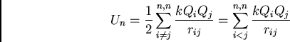 |
(20) |
In these expressions each pair interaction is counted once
and the total potential energy is the sum of the potential
energies of all pairs.
Next: About this document ...
Phillip Duxbury
2002-09-10