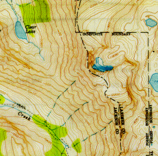
For instance consider the map on the right of the Rawah Wilderness in northern Colorado . All points on the same line are at the same elevation, just as all points on the same equipotential line are at the same voltage. Water flows downhill, so the rivers are always perpendicular to the contour lines on the topographic map. This is similar to the way electric field lines are always perpendicular to equipotential lines. When contour lines are close together, the slope is steep, e.g. a cliff, just as close equipotential lines indicate a strong electric field. Lakes are at the same elevation, in the same way conductors are at the same potential. |
|
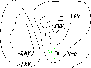 The figure to the left
shows equipotential lines. The electric field at
point a can be found by calculating the
slope at a: The figure to the left
shows equipotential lines. The electric field at
point a can be found by calculating the
slope at a:
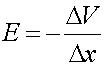
where
|
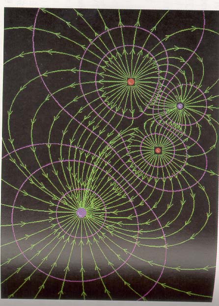
Rules for equipotential lines:
- Electric field lines are perpendicular to the equipotential lines, and point "downhill": from higher potential toward lower.
- A conductor forms an equipotential surface.
- Where equipotential surfaces are close to each other, the electric field is strong.