Bob Stein's Research Projects Solar Surface Magneto-Convection Supergranule scale Convection Magnetic Flux Emergence Active Region Formation Meso-granule scale Magneto-Convection Numerical Method Simulation Results Simulation vs. Observations Oscillations Mode spectrum Mode frequencies Mode asymmetry Time-Distance Anaylsis Mode Driving and Damping Radiation - Hydrodynamics Chromospheric dynamics and structure Dynamic line formation Publications Talks Simulation Data

Realistic Solar Surface Convection

Our goal is to understand convection in the solar envelope: its role in transporting energy and angular momentum, in generating the solar magnetic field, in providing energy to heat the solar chromosphere and corona, and interacting with waves and oscillations.

This goal is pursued by studying the results of realistic simulations of magneto-convection near the solar surface in collaboration with Åke Nordlund (Copenhagen University), Mats Carlsson, Viggo Hansteen and Boris Gudiksen (Oslo University), Junwei Zhao (Stanford University) and Dali Georgobiani. [See "Validation of Time-Distance Helioseismology by use of Realistic Simulations of Solar Convection", Astrophys. J., 659, 848-857, (2007); "Solar Small Scale Magneto-Convection", Astrophys. J., 642, 1246-1255, (2006); "Observational manifestations of solar magneto-convection --- center-to-limb variation", Astrophys. J., 610, L137, (2004); "Excitation of Radial P-Modes in the Sun and Stars", Solar Phys., 220, 229, (2004); "Simulations of Solar Granulation: I. General Properties'', Astrophys. J., 499, 914-933, (1998); "Formation of Calcium H and K Grains", Astrophys. J., 481, 500, (1997)]

Supergranule Scale Convection

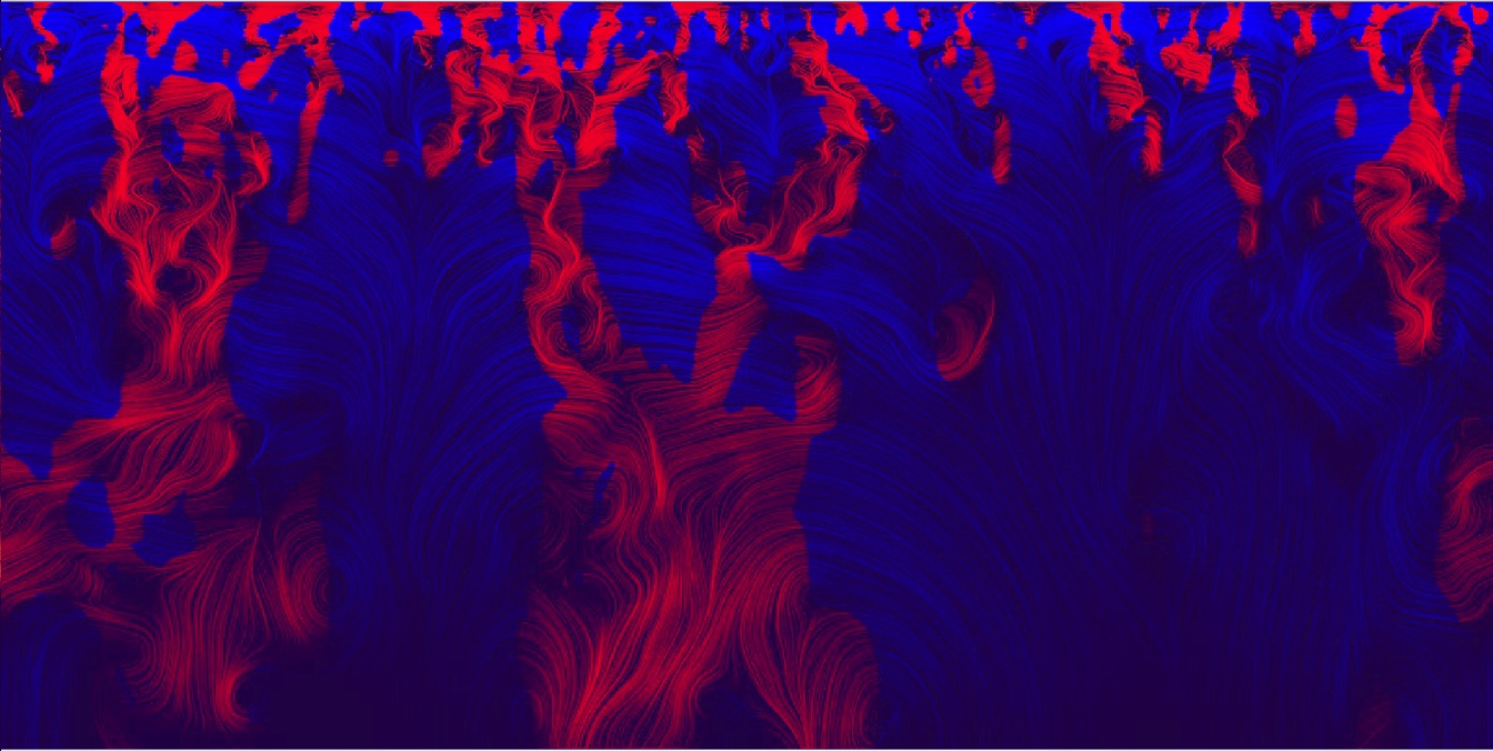
Movie (89 Mb) of Velocity and streamlines in vertical slice. Duration is 15 hours. Scale is 48 Mm wide x 20 Mm deep. Red are downflows and blue are upflows. (courtesy Chris Henze, NASA)

At the top are the granules. Deeper down are larger structures. Downflows are swept sideways and merged by the diverging upflows from below. Some downflows are halted, beating there way down against the upflows. Flow topology changes rapidly near the surface and very slowly at large depth.

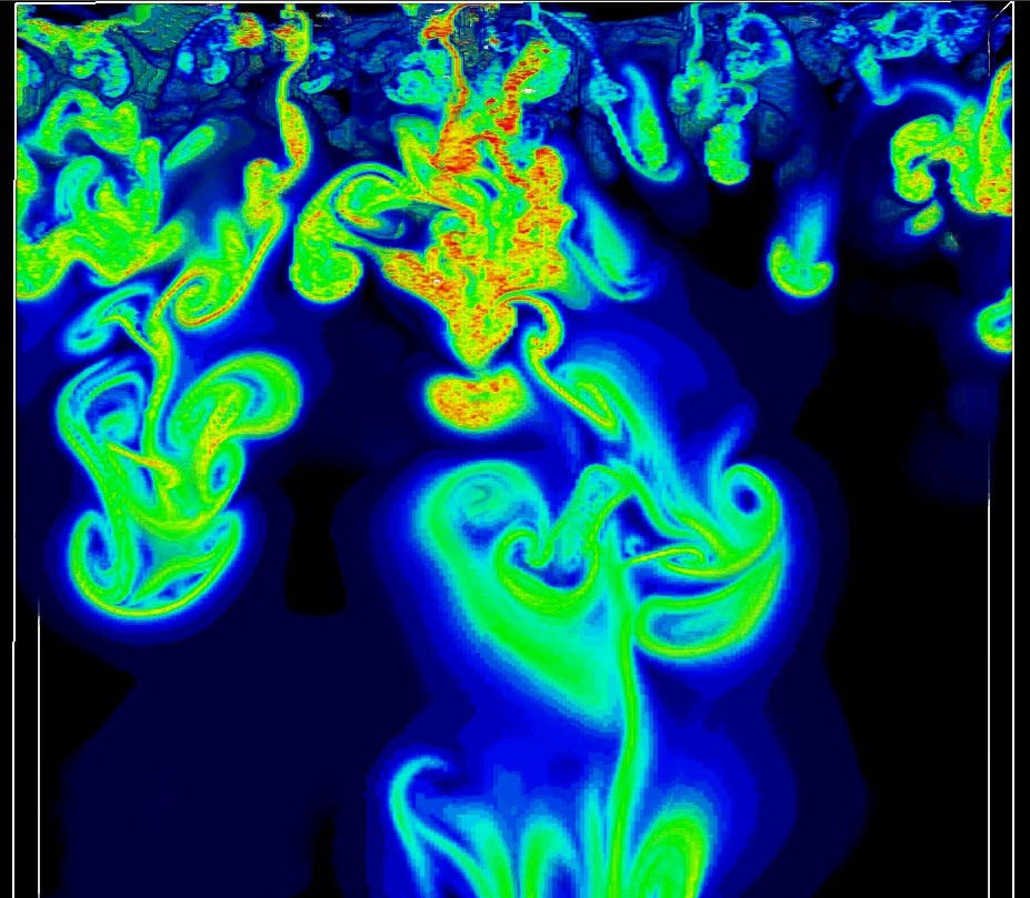
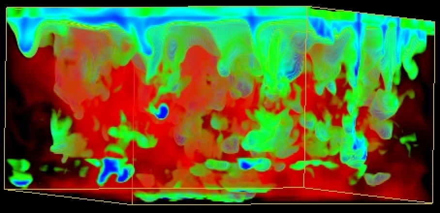
Movie (136 Mb) shows the Finite Time Lyapunov Exponent Field, which closely corresponds to the vorticity, for a time interval of 11.75 hours, in a subdomain 21 Mm wide x 19 Mm high x 0.5 Mm thick, from a 48x48 Mm wide by 20 Mm deep simulation. (Courtesy Bryan Green (AMTI/NASA).)

The size of convective cells increases with depth in order to conserve mass as the scale height becomes larger with the increasing temperature.

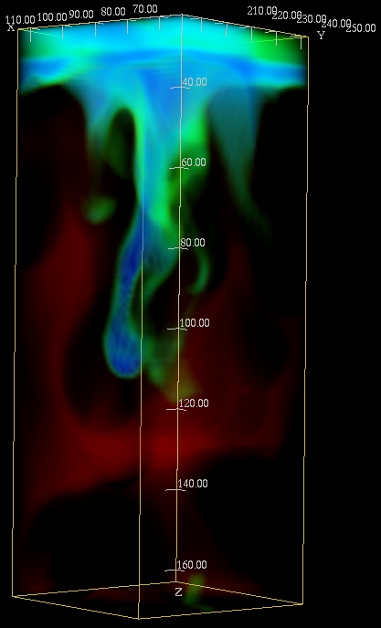
Velocity slices

Movie (400 Mb) of the vertical velocity scaned in depth. The images show the velocity at the visible surface (top left) and 2, 4, 8, 12, and 16 Mm below the surface. Each slice is 48 Mm square. Green and blue are upflows, while yellow and red are downflows. The downflows occur in more or less connected lanes surrounding compact upflow cells -- a granule at the surface and continuously larger cells with increasing depth below the surface. There are no special mesogranule or supergranule scales.

Emerging Magnetic Flux Simulations

We have simulated the emergence of magnetic flux through the solar surface. Horizontal magnetic flux is is advected by inflows into the computational domain 20 Mm below the surface. Upflows and magnetic buoyancy carry the flux to the surface. Dowflows push it down. This produces loop like structures on many different scales because the size of the upflow regions and separation of the downflows decreases as the surface is approached from below.

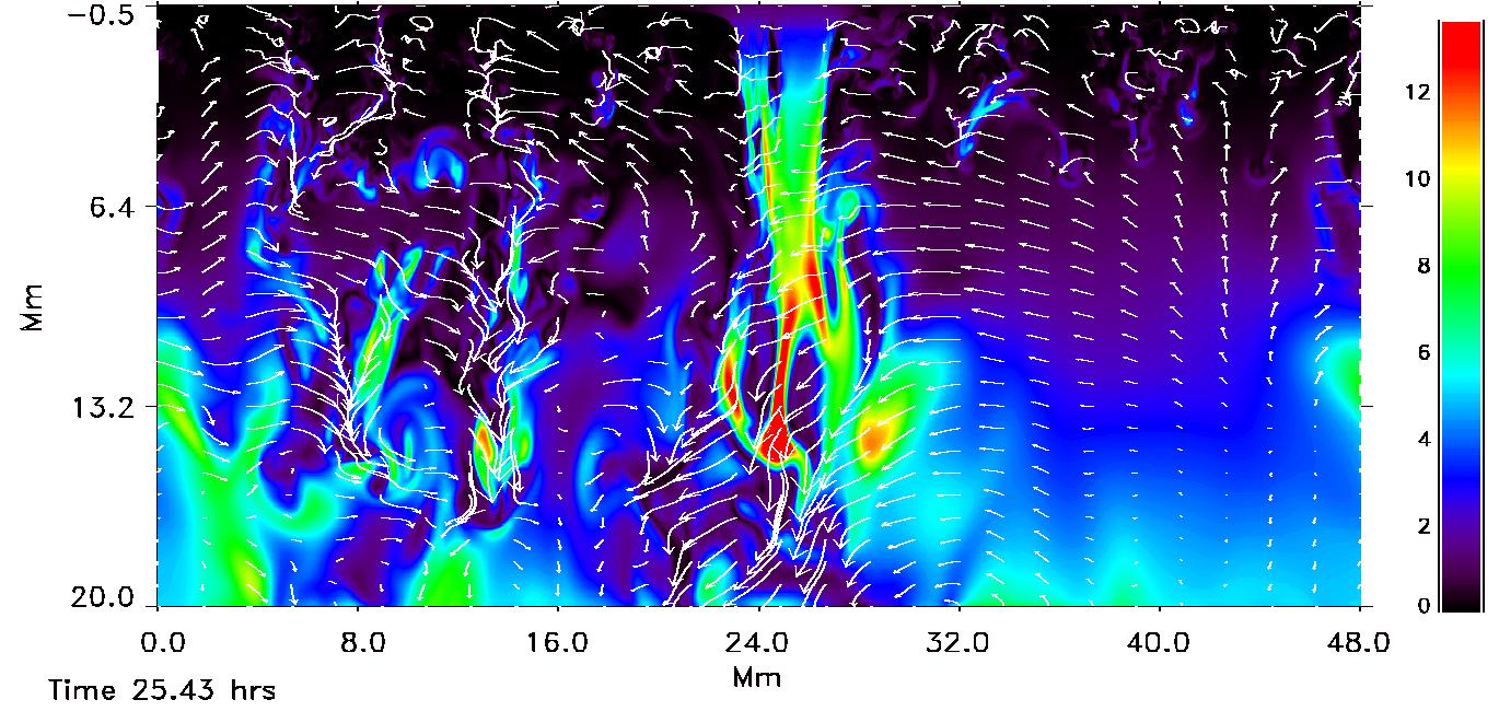
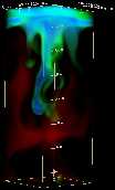
Movie (264 Mb) of magnetic flux rising to the surface from 20 Mm depth. Color is |B| in kG. White arrows are scaled velocity field. The inflow horizontal field at 20 Mm depth was gradually increased in strength with a 5 hour e-folding time until it reached 5 kG and then held fixed from that time forward.

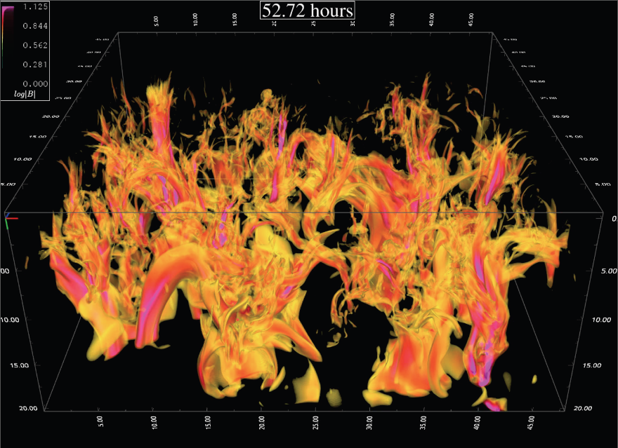
Movie (164 Mb) of log(B). The overall impression is one of magnetic field moving downward. However, rising loops can also be clearly followed. As they rise some loops become filamentary. Where loops pass through the upper boundary they leave behind their vertical legs. Where theses become concentrated pores and spots form.

Simulation results are found here.

Active Region Formation

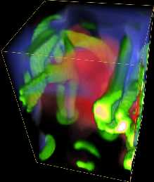
A small active region forms from a large subsurface magnetic loop produced by convective motions (see movie above) from uniform, horizontal, untwisted magnetic field of 1 kG strength at an angle of 30^o to the east-west x-axis that is advected by upflows into the computational domain at 20 Mm depth. Magnetic field first appears as small bipoles with mixed polarity. The opposite polarities separate over time into unipolar flux concentrations which become pores. The leading pore is more conentrated than the following pores and is rotating. The total unsigned vertical magnetic flux at the end is of order 10²¹ Mx.

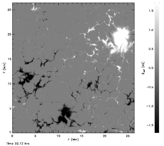
Movie (47 Mb): Vertical magnetic field. The images is clipped at 1.7 kG; the actual range is 3 kG at optical depth 0.1. Time is since uniform, untwisted, horizontal field started being advected into the convective domain.

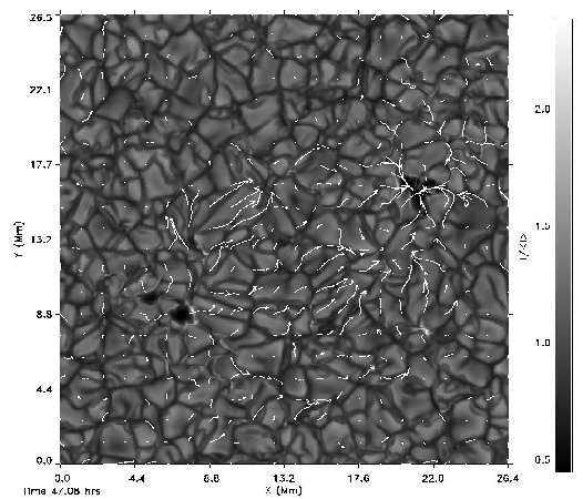
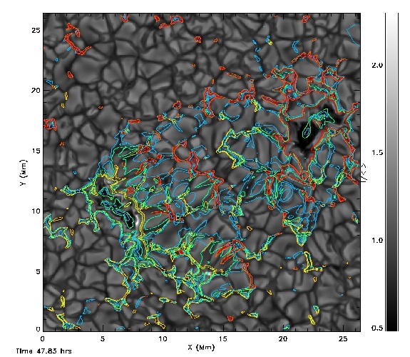
Movie (202 Mb): Emergent intensity with superimposed contours of vertical field at continuum optical depth 0.1 at levels 100G and 1.5kG. Initial active region froms in upper right. Later another active region begins to form near the bottom center. Intensity is clipped at I/avg(I) = [0.5,2]. Actual range is [0.2,2.5].

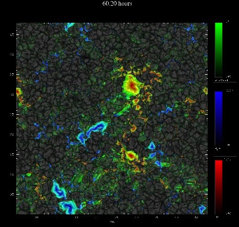
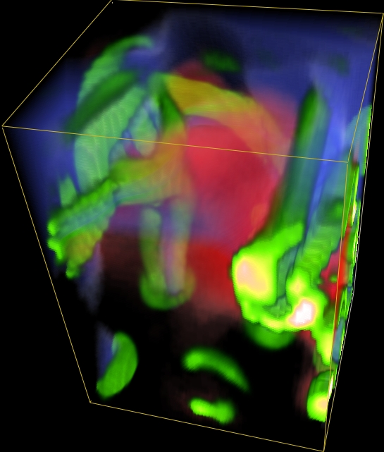
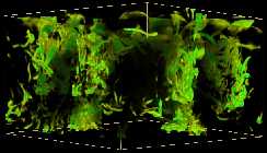
Movie (97 Mb): Magnetic field components (red vertical down, blue vertical up, green horizontal) at average continuum optical depth 0.1. Extremes of the magnetic field have been clipped. Actual extent is vertical 1.8 kG and horizontal 1.3 kG. The field emerges in localized areas as horizontal field over granules with opposite polarity vertical fields at the end points of the loop in the intergranular lanes. The horizontal field either rises through the upper boundary and disappears or is swept into the intergranular lanes. Due to the underlying large scale loop, opposite polarity field counter streams into unipolar concentrations and forms pores and spots.

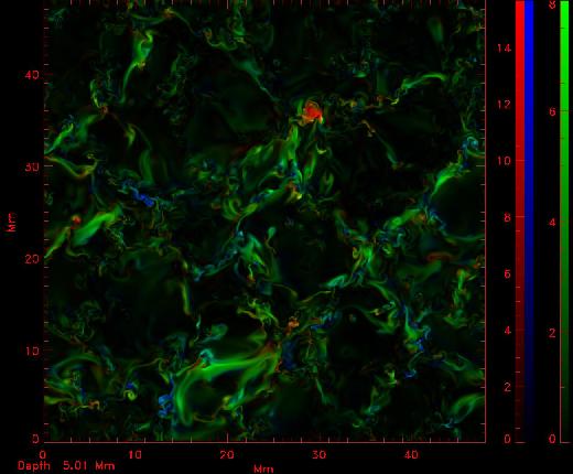
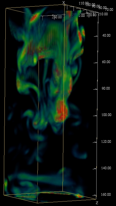
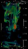
Movie (57 Mb): Depth scan of vertical (red and blue) and horizontal (green) magnetic fields (scale in kG) at a time when the first active region is well formed and the new active region in the bottom center is beginning to form. The loops from which the active regions form as visible as green horizontal field concentrations below the surface.

Movie (59 Mb): Continuum intensity image with horizontal magnetic field vectors. The intensity is clipped at I/avg(I)=[0.5,2.3] in order to clearly show the quiet Sun. The actual range is [0.2,2.5].

Movie (157 Mb): Continuum intensity image with contours of vertical (red and orange) and horizontal (green and blue) contours at 200 and 400 G. The intensity is clipped at I/avg(I)=[0.5,2.3] in order to clearly show the quiet Sun. The actual range is [0.2,2.5].

Meso-Granular Scale Magneto-Convection

Movie (47 Mb) emergent intensity from magneto-convection simulation showing center to limb variation (courtesy Mats Carlsson).

Granules appear hilly when viewed toward the limb because they really are. Hot granules emit their radiation higher up than cool intergranular lanes.

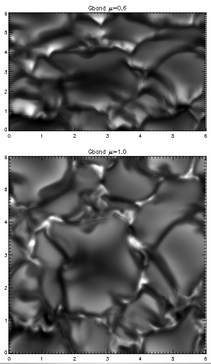
Movie (9 Mb) of G-band intensity at disk center and mu=0.6 from magneto-convection simulation (courtesy Mats Carlsson).

Small, strong magnetic field concentrations appear bright because their density is lower (to maintain pressure balance with their surroundings) so one sees deeper into the Sun where it is hotter. Towards the limb, when one looks through a low density, low opacity magnetic concentration one sees radiation from the hot granule walls behind, which is called faculae.

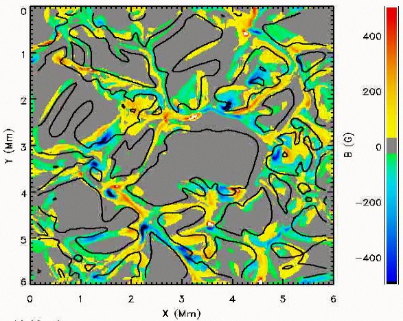
Movie (15 Mb) of magnetic field being swept into the intergranular lanes by the diverging upflows in granules and underlying larger flows.

Numerical Method

Solve the equations for conservation of mass, momentum and internal energy, plus the induction equation for the magnetic field in conservative form, on a staggered grid. Use 6th order finite difference spatial derivatives, 5th order interpolation, 3rd order Runge-Kutta time integration.

Essential physics:

Convection Simulations

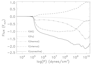
Mean Atmosphere

Topology controlled by mass conservation.
To conserve mass as it enters lower density layers, ascending fluid diverges and turns over into a downflow in approximately a scale height. Convective flow is like a fountain. It is consists of warm, broad, fairly laminar, slow upflows, surrounded by cool, narrow, turbulent, fast downdrafts. The horizontal size of the upflow cells decreases as the as the scale height decreases approaching the surface. Only a small fraction of ascending fluid actually reaches the surface.

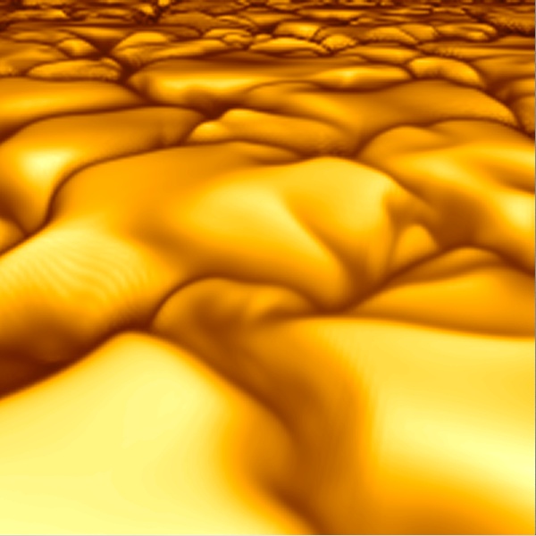
A granule. The top surface shows the emergent intensity. The interior colors show the temperature and the arrows show the flow velocity. A granule resembles a fountain. Hot fluid rises in the center and is diverted horizontally into the intergranule lanes by excess pressure over the granules. Fluid that reaches the surface cools, loses entropy, and forms the cores of the downdrafts.

Convection is driven by radiative cooling in a thin surface thermal boundary layer produces low entropy gas that forms the cores of downdrafts.

Convection is inherently non-local. The low entropy downdrafts, produced by radiative cooling in the surface thermal boundary layer, generate most of the buoyancy work that drives the convection: both large scale cellular flows and small scale turbulent motions.

movie (127 Mb)

Entropy fluctuations and mean value.

Entropy fluctuation histogram.

Movie of entropy fluctuations in a downdraft (31 Mb)
(1.2 Mm)² x 2.5 Mm deep

Convection characterized by turbulent downdrafts and smooth upflows, not hierarchy of eddies.

Vorticity primarily in intergranular lanes and downdrafts.

Movie of vorticity in same downdraft as entropy above (31 Mb)
(1.2 Mm)² x 2.5 Mm deep

vorticity movie showing ring vortex and trailing vortex tubes (127 Mb)

Horizontal scale increases with increasing depth, also because of mass conservation.
No distinct mesogranular or supergranular cell size.

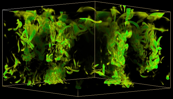
Vorticity slices

The top slice shows vortex tubes at the surface viewed from above. The dark areas are free of significant vorticity and correspond to the hot, upflowing, bright granules. The vortex tubes are concentrated in the cool, downflowing, dark intergranule lanes. The twisting of these vortices about one another shows the turbulent nature of the flow.

At increasing depth, lower slices, the vorticity becomes confined to the boundary of the mesogranule and the large upflow cell in the interior of the mesogranule is nearly vorticity free.

Simulation vs. Observations

Convection

Granulation (visible continuum).

Emergent Intensity

The emergent intensity in the simulation (top) is very similar to the observed solar intensity (bottom) when the simulation results are smoothed with a modulation transfer function to represent the effects of the telescope and atmospheric seeing (middle). The observations are from the Swedish Solar Observatory on La Palma, courtesy of the Lockheed Palo Alto Research Center.
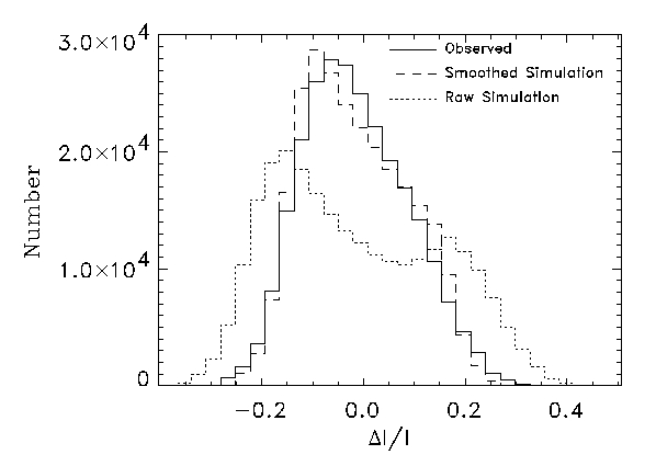
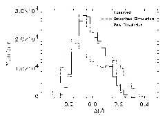
Size Spectrum

But beware: any image with sharp edged features (such as ) produces such a distribution.
Emergent intensity distribution (visible continuum).
Photospheric line profiles (visible)
( "Line formation in solar granulation. I. Fe line shapes, shifts and asymmetries", Asplund, M., Nordlund, Å., Trampedach, R., Allende Prieto, C. and Stein, R. F., Astron. and Astroph., 359, 729-742, 2000)
Line Formation: Fe I+II lines
- Accurate wavelengths and gf-values
- No free parameters (no micro- or macroturbulence, damping enhancement, etc)
Line widths, shifts, and shapes provide constraints
- Width <-> flow velocity (thermal speed is small)
- Shift <-> temperature-velocity correlations
- Shape <-> details of convective overshoot, cf bisectors
Excellent agreement exists between simulated and observed profiles of weak and intermediate strength FeI and FeII lines.
Without the convective and wave velocities, the line profiles would differ drastically from the observed profiles:

Including velocities and sufficient resolution, produces close agreement between simulated and observed profiles:
2D simulations do not give observed profiles

The average profile is a combination of profiles with very different shifts, widths and shapes. (Thick red line is average profile)

Line shapes depend on the details of the convection overshooting and are revealed in the line bisectors.
Small differences exist between synthetic and observed profiles for strong FeI lines. These can be used to improve the physics of the upper photosphere (and chromosphere).
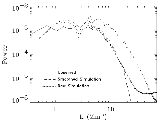
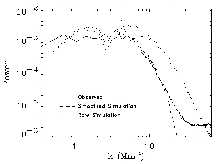
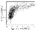
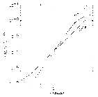
Velocity Spectrum
The simulation velocity spectrum fits almost exactly with the observed velocity spectrum from MDI and TRACE. This shows that our simulations have the correct velocity amplitude and at large scales the correct spectrum.

Agreement with observations gives confidence in model of convection

Solar P-Mode Oscillations

Mode Spectrum

k-omega diagram. The simulations excite a rich spectrum of p-mode oscillations (left), very similar to the MDI diagram (right). The dark line is the theoretical f-mode.

Mode Frequencies
( "Convective contributions to the frequencies of solar oscillations", Rosenthal, C. S., Christensen-Dalsgaard, J., Nordlund, Å., Stein, R. F., Trampedach, R., Astron. and Astrophys. 351, 689-700, 1999)
Acoustic eigenmodes of the atmosphere in our simulation are excited. We can study the properties of these simulation p-modes to understand the solar p-modes better.
The mean atmosphere from the simulations gives p-mode eigenfrequencies in better agreement with observed modes than standard, spherically symmetric, mixing-length models.
Standard, 1-D, Spherically Symmetric, Mixing Length Model

3D Convection Simulation + Mixing Length Envelope Extension

High frequency modes' cavity is enlarged by

turbulent pressure support (convergence to correct value ensured by line widths)

3D radiative transfer effects
Don't see hot gas. Average temperature higher for a given effective temperature

Contribute equally to elevating photosphere by 150 km.

High frequency modes' frequency is reduced.
Remaining discrepancies in mode frequencies can now be used to investigate details of the dynamical interaction of p-modes with convection.
Mode Asymmetry (helioseismology).
P-mode spectrum is asymmetric. Velocity power is larger toward low frequencies and Intenstiy power is larger toward high frequencies.
( "Numerical Simulations of Oscillation Modes of the Solar Convection Zone", Georgobiani, D. Kosovichev, A.G., Nigam, R., Nordlund, Å, Stein, R.F. Astrophys. J., 530, L139-L142, 2000)

Intensity-Velocity phase jumps at modes.
Time-Distance Diagram (helioseismology)

Time - Distance diagram. The simulation and mdi time-distance diagrams are similar. Dark line is the theoretical td-diagram. (courtesy Junwei Zhao)
P-mode Excitation (helioseismology).
( "Solar Oscillations and Convection: II. Excitation of Radial Oscillations", Stein, R. F. and Nordlund, Å., Astrophys. J., 546, 585-603, 2001)
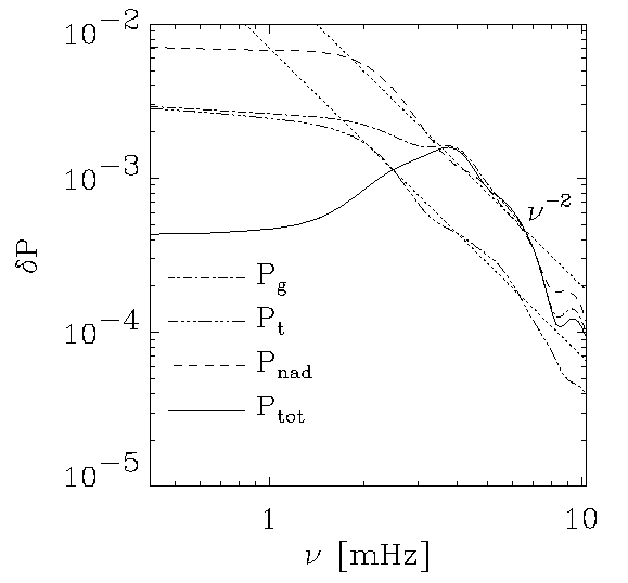
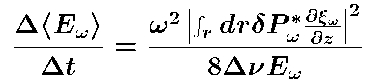
Stochastic, non-adiabatic, gas and turbulent pressure fluctuations excite the p-modes via PdV work,

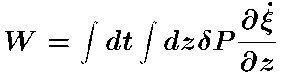
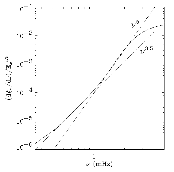
Mode excitation rate is,

Driving decreases at low frequencies because the mode compression decreases and the mode mass increases.

Driving decreases at high frequency because the pressure fluctuations decrease.

Driving occurs closer to the surface at higher frequencies

Logarithm (base 10) of the work integrand as a function of frequency and depth (in unites of erg/cm²/s).
Driving occurs in the intergranular lanes and at the edges of granules.

Non-adiabatic pressure fluctuations at 100 km depth in the 2 - 5 mHz range, with the contours of zero velocity at the surface to outline the granules. The units of the pressure fluctuations are 10³ dyne cm_$-2. In this frequency range, where the driving is maximal, the largest pressure fluctuations occur at the edges of granules and inside the intergranular lanes.

Radiation - Hydrodynamics

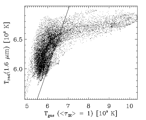
Mats Carlsson (Oslo University) and I have performed self-consistent non-LTE radiation hydrodynamics simulations of the propagation of acoustic waves through the solar chromosphere. We find that the chromosphere is dynamic and that static diagnostics do not accurately represent its properties. For instance, enhanced chromospheric emission, which corresponds to an outwardly increasing semi-empirical temperature structure, can be produced by wave motions without any increase in the mean gas temperature. This is because in the ultraviolet and visible the Planck function depends exponentially on the temperature, so the emission tends to represent the temperature maxima rather than the mean values. Thus, despite long held beliefs, the sun may not have a classical chromosphere in magnetic field free internetwork regions (``Does a Non - Magnetic Solar Chromosphere Exist?'', Carlsson & Stein, Ap. J. Lett., 440, L29 (1995)).

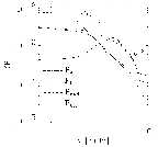
Chromospheric Temperature

Time averaged (Mean) gas temperature in the dynamical simulation and the Semi-empirical temperature that gives the best fit to the time average of the intensity as a function of wavelength calculated from the dynamical simulation. Also shown are: the minimum and maximimum (range) temperatures in the simulation, the starting model temperature, and the semi-empirical model of Fontenala, Avrett & Loeser, 1993. The semi-empirical model giving the same intensities as the dynamical simulation shows a chromospheric temperature rise while the mean temperature in the simulation does not.

We have also simulated the generation of CaII H_2V bright grains by acoustic shocks. The bright grains are produced by shocks near 1 Mm above tau₅₀₀=1. The asymmetry of the line profile is due to velocity gradients.

The formation of the CaII H_2V bright grains. The contribution function to intensity (lower right) and the factors entering its calculation, opacity and optical depth (upper left), Source function (upper right) and tau*exp(-tau) (lower left). The functions are shown as grey-scale images as functions of frequency in the line (in velocity units) and height in the atmosphere. All panels also show the velocity as a function of height (with upward velocity positive to the left in the figure) and the height where tau=1 (grey line). The top right panel, in addition, shows the Planck function (dotted) and the source function (dashed), with high values to the left. The source function (image, upper right panel) is constant across the line at a given height, because of the assumption of CRD, and is substantially below the Planck function above 1 Mm due to the non-LTE decoupling. The bottom right panel also shows the emergent intensity as a function of frequency.

The simulations closely match the observed behavior of CaII H_2V bright grains down to the level of individual grains ( "Formation of Calcium H and K Grains", Carlsson, M. and Stein, R. F., Astrophys. J. 481, 500, 1997).

The crucial lesson to learn from these studies is that the chromosphere is Dynamic and a static analysis may not give correct results, ( "The New Chromosphere", Carlsson, M. and Stein, R. F., in New eyes to see inside the sun and stars : pushing the limits of helio- and asteroseismology with new observations from the ground and from space, IAU Symposium 185, eds. F. L. Deubner, J. Christensen-Dalsgaard and D. Kurtz, (Kluwer:Dordrecht) 435-446, 1998, and "Dynamic Behavior of the Solar Atmosphere", Stein, R. F. and Carlsson, M., in Solar Convection and Oscillations and their Relationship, eds. F.P.Pijpers, J. Christensen-Dalsgaard, C. Rosenthal, (Kluwer:Dordrecht), 261-276, 1997).

This research is/was supported by NASA grants NNX07AO71G, NNX07AH79G, NNX08AH44G, and NSF grant AST-0605738. The calculations were performed on the NASA Advanced Supercomputing Division "Pleiades" computer. Any opinions, findings, and conclusions expressed in this material are those of the author(s) and do not necessarily reflect the views of NASA or the NSF.

This page has been accessed times.

Updated:

Bob Stein's home page, email: stein@pa.msu.edu

Supergranule Scale Convection

Emerging Magnetic Flux Simulations

Meso-Granular Scale Magneto-Convection

Essential physics:

Simulation vs. Observations

Emergent Intensity

Chromospheric Temperature